Worked examples on complex numbers and linear algebra
Table of Contents
- Introduction.
- Complex numbers
- Addition of complex numbers
- Subtraction of complex numbers
- Multiplication of two complex numbers:
- Conjugate of a complex number
- Modulus of a complex number
- Quotient of two complex numbers:
- Modulus, argument Euler's formula and polar form.
- Compute n-th roots of a complex number
- Compute n-th power of a complex number (Moivre's Formula)
- Geometry in the complex plane:
- Matrix arithmetic
- The identity matrix
- Determinants
- Inverse of a square matrix
- System of linear equations
- Linear transformations between vector spaces
- The kernel, Image, rank and nullity
- The dimension theorem
- Eigenvalues and eigenspaces
- Diagonalizable matrix
- The Gram–Schmidt algorithm
- Multiplication by scalar and addition of vector in \(\mathbb{R}^n\).
- Definition of Linearly dependent and Linearly independent set of vectors.
- Inner product of two vectors in \(\mathbb{R}^n\)
- Geometric interpretation of the inner product (Angle between two vectors)
- Equation of a hyperplane in \(\mathbb{R}^n\)
- The cross product in \(\mathbb{R}^3\)
- Complex numbers
- References
© 2024 Daniel Ballesteros Chávez
This work is licensed under CC BY 4.0![]()
![]()
Introduction.
These notes contain a series of worked examples and exercises for students of engineering who are taking a first course in Linear Algebra at Poznan University of Technology.
The idea is to provide the students with enough examples on the computational side of the subject, so they can practice and improve their skills. These exercises also work as a source of examples for definitions, propositions and theorems behind the theory of this useful and beautiful subject.
We hope that this material can complement the tutorial sessions, where sometimes it is not possible to present fully step-by-step solutions to exercises that involve lengthy computations due to time limitations.
Introduction to Linear Algebra is the opening gate to a whole new world of mathematical tools with countless applications including geometry, graph theory, circuits and much more.
I would like to express my gratitude to the students that took part in the course for their remarks, suggestions and discussions.
I take responsibility for any mistake/typo that may appear in the notes and any notice will be very appreciated.
Complex numbers
The set of complex numbers
\begin{equation*} \mathbb{C}= \{ x + iy : x,y\in \mathbb{R}, i^2 = -1\} \end{equation*}The set of complex numbers is denoted by \(\mathbb{C}\). Every element \(z\in \mathbb{C}\) can be written as
\begin{equation*} z = x + i y, \end{equation*}where \(x,y\in \mathbb{R}\) and \(i\) is a special complex number with the property that \(i^2 = -1\).
On this set, the operations of addition, subtraction, multiplication and division are defined.
Addition of complex numbers
If \(z = x_1 + i y_1\) and \(w = x_2 + i y_2\) are two complex numbers, then the sum is
\begin{equation*} z + w = (x_1 + x_2) + i(y_1 + y_2). \end{equation*}- Example
Let \(z = 4 + \frac{i}{4}\) and \(w = 3 - 5i\). Then, the sum is
\begin{equation*} \begin{split} z + w & = \left( 4 + \frac{i}{4} \right) + (3 - 5i) \\ & = \left( 4 + 3 \right) + \left(\frac{i}{4} - 5i\right) \\ & = 7 + i \left(\frac{1}{4} - 5\right) \\ & = 7 - \frac{19}{4} i\\ \end{split} \end{equation*}Subtraction of complex numbers
If \(z = x_1 + i y_1\) and \(w = x_2 + i y_2\) are two complex numbers, then the difference is
\begin{equation*} z - w = (x_1 - x_2) + i(y_1 - y_2). \end{equation*}- Example
Let \(z = 7 - \frac{3i}{2}\) and \(w = 1 - i\). Then
\begin{equation*} \begin{split} z - w & = \left( 7 - \frac{3i}{2} \right) - \left(1 - i \right) \\ & = 7 - \frac{3i}{2} - 1 + i \\ & = 6 - \frac{i}{2} \end{split} \end{equation*}Multiplication of two complex numbers:
If \(z = x_1 + i y_1\) and \(w = x_2 + i y_2\) are two complex numbers, then the multiplication or product is
\begin{equation*} z w = (x_1x_2 - y_1y_2) + i(x_1y_2 + x_2y_1). \end{equation*}- Example
Let \(z = 7 - \frac{3i}{2}\) and \(w = 1 - i\). Then
\begin{equation*} \begin{split} z w & = \left( 7 - \frac{3i}{2} \right) \left(1 - i \right) \\ & = 7 - 7i - \frac{3i}{2} + \frac{3}{2} i^2 \\ & = 7 - 7i - \frac{3i}{2} - \frac{3}{2} \\ & = \frac{11}{2} - \frac{17i}{2}. \end{split} \end{equation*}Conjugate of a complex number
If \(z = x + iy\), then the conjugate is
\begin{equation*} \overline{z} = x - iy. \end{equation*}- Examples
- The conjugate of \(z = 3 - 7i\) is \(\overline{z} = 3 + 7i\).
- The conjugate of \(z = 1 + 3i\) is \(\overline{z} = 1 - 3i\).
- The conjugate of \(z = 3i\) is \(\overline{z} = -3i\).
- The conjugate of \(z = 5\) is \(\overline{z} = 5\).
Modulus of a complex number
If \(z = x + iy\), then modulus of \(z\) is the positive real number
\begin{equation*} \, |z| =\sqrt{ x^2 + y^2}. \end{equation*}- Example
- The modulus of \(z = 3 - 7i\) is the real number \(|z| = \sqrt{58}\).
- Compute the modulus of \(z = \frac{1}{2} + \sqrt{2} i\).
- Example
- Notice that for any \(z = x + iy\), the product of a complex number with its conjugate equals the modulus squared:
Quotient of two complex numbers:
If \(z = x_1 + i y_1\) and \(w = x_2 + i y_2\) are two complex numbers with \(w \neq 0\), then the quotient is
\begin{equation*} \frac{z}{w} = \frac{z}{w} \frac{\overline{w}}{\overline{w}} = \frac{(x_1 + i y_1)(x_2 - iy_2)}{x_2^2 + y_2^2}. \end{equation*}- Example
- Write the following quotient of complex number in the form \(x + i y\).
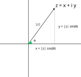
Modulus, argument Euler's formula and polar form.
Every complex number can be written in polar form
\begin{equation*} z = r e^{i\theta}, \end{equation*}where
- \(r = |z|\) is the modulus of the complex number.
- \(\theta\) is the argument of the complex number (angle).
- \(e^{i\theta} = \cos(\theta) + i \sin(\theta)\) is the beautiful Euler's formula.
- Example
- Write in polar form the complex number \(z = -1 -\sqrt{3}i\).
A direct computation shows that the modulus is
\begin{equation*} r = |z| = \sqrt{(-1)^2 + (-\sqrt{3})^2} = \sqrt{4} =2. \end{equation*}After you draw the complex number on the plane, you can choose verify that
\begin{equation*} \theta = \pi + \frac{\pi}{3} = \frac{4\pi}{3}. \end{equation*}Then we can write:
\begin{equation*} z = 2 e^{\frac{4\pi}{3} i}, \end{equation*}or equivalently
\begin{equation*} z = 2 \left( \cos\left(\frac{4\pi}{3}\right) + i\sin\left(\frac{4\pi}{3}\right)\right). \end{equation*}Compute n-th roots of a complex number
If \(z = r e^{i\theta}\), then the nth-root is given by the formula
\begin{equation*} \sqrt[n]{z} = \sqrt[n]{r}\left( \cos\left(\frac{\theta + 2k\pi}{n}\right) + i\sin\left(\frac{\theta + 2k\pi}{n}\right)\right), \end{equation*}and there are n-different values corresponding to \(k = 0, 1, 2, ..., (n-1)\).
- Example
- Compute \(\sqrt[3]{-2+2i}\).
The modulus of \(-2 + 2i\) is \(r = \sqrt{8}\), and the argument is \(\theta =\frac{3\pi}{4}\).
Notice that \(\sqrt[3]{r} = \sqrt[3]{\sqrt{8}} = (8)^{1/6} = (2^3)^{1/6} = 2^{1/2} = \sqrt{2}\).
Then using the identity from the definition
\begin{equation*} \sqrt[3]{-2+2i} = \sqrt{2} \left( \cos\left(\frac{\frac{3\pi}{4} + 2k\pi}{3}\right) + i\sin\left(\frac{\frac{3\pi}{4} + 2k\pi}{3}\right)\right), \end{equation*}The root for \(k=0\) is
\begin{equation*} \begin{split} z_0 & = \sqrt{2} \left( \cos\left(\frac{3\pi}{12}\right) + i\sin\left(\frac{3\pi}{12}\right)\right)\\ & = \sqrt{2} \left( \cos\left(\frac{\pi}{4}\right) + i\sin\left(\frac{\pi}{4}\right)\right)\\ & = \sqrt{2} \left( \frac{1}{\sqrt{2}} + i \frac{1}{\sqrt{2}}\right)\\ & = 1 + i. \end{split} \end{equation*}The root for \(k=1\) is
\begin{equation*} \begin{split} z_1 &= \sqrt{2} \left( \cos\left(\frac{11\pi}{12}\right) + i\sin\left(\frac{11\pi}{12}\right)\right), \end{split} \end{equation*}The root for \(k=2\) is
\begin{equation*} \begin{split} z_2 &= \sqrt{2} \left( \cos\left(\frac{19\pi}{12}\right) + i\sin\left(\frac{19\pi}{12}\right)\right), \end{split} \end{equation*}Compute n-th power of a complex number (Moivre's Formula)
If \(z = re^{i\theta}\) then
\begin{equation*} z^n = r^ne^{in\theta}. \end{equation*}Equivalently we can write the so called Moivre's formula:
\begin{equation*} z^n = r^n\left( \cos\left(n\theta\right) + i\sin\left(n\theta\right)\right). \end{equation*}- Example
- Compute \((-2+2i)^4\).
The modulus of \(-2 + 2i\) is \(r = \sqrt{8}\), and the argument is \(\theta =\frac{3\pi}{4}\), then
\begin{equation*} (-2 + 2i)^4 = 8^2\left( \cos\left(3\pi\right) + i\sin\left(3\pi\right)\right) = -64. \end{equation*}Geometry in the complex plane:
We should understand the modulus of a complex number as a length:
- Length of line segment
- \(|z_1 - z_0|\) measures the length of the line segment joining the two given complex numbers \(z_0\) and \(z_1\).
- Circle
- For a given \(z_0\), the set of complex numbers satisfying \(|z- z_0| = R\) describes the circle with centre at \(z_0\) and radius \(R\).
- Ellipse
An ellipse is a plane curve surrounding two focal points, such that for all points on the curve, the sum of the two distances to the focal points is a constant.
\begin{equation*} \, |z - a_1| + |z - a_2| = c, \quad \mbox{as long as } c > |a_1 - a_2|. \end{equation*}- Hyperbola
- (Exercise)
- Perpendicular bisector
Perpendicular bisector of the line segment joining two complex numbers \(z_1\) and \(z_2\)
\begin{equation*} \,|z - z_1| = |z - z_2| \end{equation*}
Matrix arithmetic
In this section we will review the basic arithmetic of matrices with real coefficients. One can easily generalise these properties for matrices with complex coefficients, and we encourage the student to write examples in this field.
Matrix with real coefficients
A matrix \(A\) of size \(n\times m\) with real coefficients, is a rectangular arrangement of real numbers consisting of \(n\) rows and \(m\) columns (in this order).
\begin{equation*} A = \left( \begin{array}{ccc} a_{11} & \cdots & a_{1m}\\ \vdots & \vdots & \vdots \\ a_{n1} & \cdots & a_{nm}\\ \end{array} \right) \end{equation*}The entries of \(A\) are the real numbers \(a_{ij}\), where \(1\leq i \leq n\) (is the row index) and \(1 \leq j \leq m\) (is the column index).
The set of all matrices with real coefficients of size \(n \times m\) will be denoted by \(\mathcal{M}^{n\times m}(\mathbb{R})\).
When the number of rows is the same as the number of columns (\(n = m\)), then \(A\) is also called a square matrix. If \(A\) is a square matrix, the diagonal of \(A\) is given by the coefficients \(a_{ii}\), for \(i = 1, 2, ...,n\), that is, \(\mbox{diag}(A) = (a_{11}, a_{22}, \ldots, a_{nn})\).
- Example
- An example of a \(3\times 3\) matrix is
- Example
- An example of a \(2\times 3\) matrix is
The entry \(b_{23} = -6\), and the entry \(b_{12} = 2\).
Multiplication by a scalar
Let \(r\in \mathbb{R}\) be any real number and \(A\) be a matrix of size \(n\times m\) with real coefficients, with entries \(a_{ij}\). We define the product of \(A\) by the sacar \(r\) as the matrix \(rA\) whose entries are \(ra_{ij}\).
\begin{equation*} A = \left( \begin{array}{ccc} a_{11} & \cdots & a_{1m}\\ \vdots & \vdots & \vdots \\ a_{n1} & \cdots & a_{nm}\\ \end{array} \right), \quad rA = \left( \begin{array}{ccc} ra_{11} & \cdots & ra_{1m}\\ \vdots & \vdots & \vdots \\ ra_{n1} & \cdots & ra_{nm}\\ \end{array} \right). \end{equation*}- Example
Sum and difference of matrices
Let \(A\) and \(B\) any two matrices of the same size \(n\times m\) with real coefficients with entries \(a_{ij}\) and \(b_{ij}\), respectively. We define the sum of \(A\) and \(B\) as the matrix \(A + B\) of the same size \(n \times m\), whose entries are \(a_{ij} + b_{ij}\). The difference \(A - B\) is the matrix of the same size \(n \times m\), whose entries are \(a_{ij} - b_{ij}\).
\begin{equation*} A = \left( \begin{array}{ccc} a_{11} & \cdots & a_{1m}\\ \vdots & \vdots & \vdots \\ a_{n1} & \cdots & a_{nm}\\ \end{array} \right), \quad B = \left( \begin{array}{ccc} b_{11} & \cdots & b_{1m}\\ \vdots & \vdots & \vdots \\ b_{n1} & \cdots & b_{nm}\\ \end{array} \right), \end{equation*} \begin{equation*} A + B = \left( \begin{array}{ccc} a_{11} + b_{11} & \cdots & a_{1m} + b_{1m}\\ \vdots & \vdots & \vdots \\ a_{n1} + b_{n1} & \cdots & a_{nm} + b_{nm}\\ \end{array} \right), \quad A - B = \left( \begin{array}{ccc} a_{11} - b_{11} & \cdots & a_{1m} - b_{1m}\\ \vdots & \vdots & \vdots \\ a_{n1} - b_{n1} & \cdots & a_{nm} - b_{nm}\\ \end{array} \right). \end{equation*}- Example
- Compute the matrix \(3A - 2B\) where
Then
\begin{equation*} \begin{split} 3A - 2B & = 3 \left( \begin{array}{rrr} 1 & 2 & 3\\ -4 & -5 & -6 \\ \end{array} \right) -2\left( \begin{array}{rrr} 0 & 3 & 9\\ -6 & -2 & 6 \\ \end{array} \right) \\ &= \left( \begin{array}{rrr} 3 & 6 & 9\\ -12 & -15 & -18 \\ \end{array} \right) -\left( \begin{array}{rrr} 0 & 6 & 18\\ -12 & -4 & 12 \\ \end{array} \right) \\ &= \left( \begin{array}{rrr} (3 -0) & (6 -6) & (9- 18)\\ (-12 + 12) & (-15 + 4) & (-18 - 12) \\ \end{array} \right) \\ & = \left( \begin{array}{rrr} 3 & 0 & -9\\ 0 & -11 & -30 \\ \end{array} \right). \end{split} \end{equation*}Transpose of a matrix
Let \(A\) a matrix of size \(n\times m\) with real coefficients with entries \(a_{ij}\). We define the transpose of \(A\) as the matrix \(A^T\) of size \(m \times n\), whose entries are \(a^{T}_{ij} = a_{ji}\).
\begin{equation*} A = \left( \begin{array}{ccc} a_{11} & \cdots & a_{1m}\\ \vdots & \vdots & \vdots \\ a_{n1} & \cdots & a_{nm}\\ \end{array} \right), \quad A^T = \left( \begin{array}{ccc} a_{11} & \cdots & a_{n1}\\ \vdots & \vdots & \vdots \\ a_{1m} & \cdots & a_{nm}\\ \end{array} \right), \end{equation*}- Example
- The transpose matrix of
is the following matrix:
\begin{equation*} A^{T} = \left( \begin{array}{rrr} 1 & -4 \\ 2 & -5 \\ 3 & -6 \\ \end{array} \right). \end{equation*}- Example
- The transpose matrix of the matrix
gives the same matrix. In this case we write: \(A^{T}= A\).
Let \(A\) be a square matrix. If \(A^{T} = A\), then we will say that \(A\) is a symmetric matrix.
Multiplication of two matrices
Let \(A\) a matrix of size \(n\times m\) with entries \(a_{ij}\) and \(B\) a matrix matrices of size \(m \times \ell\) with entries \(b_{ij}\). We define the product of \(A\) with \(B\) (in that order) as the matrix \(AB\) of size \(n \times \ell\) with entries \(C_{ij}\), with \(1 \leq i \leq n\), \(1 \leq j \leq \ell\) given by
\begin{equation*} c_{ij}= \sum_{k = 1}^{m} a_{ik}b_{kj}. \end{equation*} \begin{equation*} A = \left( \begin{array}{ccc} a_{11} & \cdots & a_{1m}\\ \vdots & \vdots & \vdots \\ a_{n1} & \cdots & a_{nm}\\ \end{array} \right), \quad B = \left( \begin{array}{ccc} b_{11} & \cdots & b_{1\ell}\\ \vdots & \vdots & \vdots \\ b_{m1} & \cdots & b_{m\ell}\\ \end{array} \right), \end{equation*} \begin{equation*} A B = \left( \begin{array}{ccc} (a_{11}b_{11} + a_{12}b_{21} + \cdots + a_{1m}b_{m1}) & \cdots & (a_{11}b_{1\ell} + a_{12}b_{2\ell} + \cdots + a_{1m}b_{m\ell}) \\ \vdots & \vdots & \vdots \\ (a_{n1}b_{11} + a_{n2}b_{21} + \cdots + a_{nm}b_{m1}) & \cdots & (a_{n1}b_{1\ell} + a_{n2}b_{2\ell} + \cdots + a_{nm}b_{m\ell}) \\ \end{array} \right). \end{equation*}- Example
- Perform the follwong multiplication of matrices
Then computing each of the entries
\begin{equation*} \begin{split} c_{11} & = (1)(-11) + (-12)(3) + (5)(-1) = - 52 \\ c_{21} & = (0)(-11) + (-2)(3) + ( 4)(-1) = - 10 \\ c_{31} & = (3)(-11) + (3)(3) + (0)(-1) = - 24 \\ c_{12} & = (1)(1) + (-12)(-2) + (5)(1) = 30 \\ c_{22} & = (0)(1) + (-2)(-2) + ( 4)(1) = 8 \\ c_{32} & = (3)(1) + (3)(-2) + (0)(1) = -3 \\ \end{split} \end{equation*}then the result is
\begin{equation*} AB = \left( \begin{array}{rrr} -52 & 30 \\ -10 & 8 \\ -24 & -3 \\ \end{array} \right). \end{equation*}The identity matrix
The square matrix \(I\) of size \(n\) is the matrix consisting of 1's in its diagonal and 0's elsewhere:
\begin{equation*} I = \left( \begin{array}{ccc} 1 & 0 & \cdots & 0\\ 0 & 1 & \cdots & 0\\ \vdots & \vdots &\ddots & \vdots \\ 0 & 0 & \cdots & 1\\ \end{array} \right) \end{equation*}- Example
- Notice that the identity matrix has the property that \(AI = I A = A\).
If we do not specify the size of the matrix \(I\), it should be clear from the context.
Determinants
The determinant is a function that assigns to a square matrix \(A\) of size \(n\), a real number \(\mbox{det}(A)\). It is a fundamental function in matrix analysis and it can be properly defined as an alternating multi-linear function, but we will leave this definition for later.
The determinant is a function \(\det : M^{n\times n} \to \mathbb{R}\) that satisfies the following properties:
- For any \(A\in M^{n\times n}\) let \(B\) the square matrix obtained from \(A\) by swapping/interchanging any two rows, then we have \(\det(A) =- \det(B)\).
- Let \(r\in \mathbb{R}\), and \(A,B,C\in M^{n\times n}\) such that the three matrices differ only in a single row \(j\). If the \(j\) row of \(C\) can be obtained by adding corresponding entries in the \(j\) th rows of \(A\) and the \(j\) th row with the \(j\) entries of \(rB\), then \[\det(C) = \det(A) + r\det(B).\]
- For any \(A\in M^{n\times n}\) we have \(\det(A) = \det(A^T)\).
We say then that the determinant is alternating with respect to permutations of rows, and that is linear on each row. The last point in the proposition indicates that we can change the word rows by columns and the properties will hold accordingly.
From the three points of the proposition one can show that
- If a matrix \(A\) has one row with all entries equal to \(0\), then \(\det(A) =0\).
- If a matrix \(A\) has two repeated rows, then \(\det(A) =0\).
- For any \(r\in \mathbb{R}\), it holds that \(\det(rA) = r^n\det(A)\).
In this section we will show by working some examples, how to compute the determinant of a matrix in an inductive way.
Determinant of a \(1\times 1\) matrix
A real number \(a\in \mathbb{R}\) can be consider as a \(1\times 1\) matrix, and in this case we define \(\mbox{det}(a) = a\).
Determinant of a \(2\times 2\) matrix
Let \(A\) be a \(2\times 2\) matrix
\begin{equation*} A = \left( \begin{array}{ll} a & b \\ c & d \\ \end{array} \right). \end{equation*}Then the determinant of \(A\) is given by the following formula
\begin{equation*} \mbox{det}(A) = \left| \begin{array}{ll} a & b \\ c & d \\ \end{array} \right| = ad - bc. \end{equation*}- Example
- Compute the determinant of the matrix
A direct computation shows
\begin{equation*} \mbox{det}(A) = (4)(2) - (-1)(-2) = 8 - 2 = 6. \end{equation*}Determinant of a \(3\times 3\) matrix
Let \(A\) be a \(3\times 3\) matrix
\begin{equation*} A = \left( \begin{array}{ccc} a & b & c\\ d & e & f \\ g & h & i\\ \end{array} \right). \end{equation*}Then the determinant of \(A\) is given by the following formula
\begin{equation*} \mbox{det}(A) = \left| \begin{array}{ll} a & b & c\\ d & e & f \\ g & h & i\\ \end{array} \right| = a \left| \begin{array}{ll} e & f \\ h & i \\ \end{array} \right| - b \left| \begin{array}{ll} d & f \\ g & i \\ \end{array} \right| + c \left| \begin{array}{ll} d & e \\ g & h \\ \end{array} \right|. \end{equation*}- Example
- compute the determinant of the following matrix
Following the formula, we get
\begin{equation*} \begin{split} \left| \begin{array}{ccc} 0 & -3 & 10 \\ -6 & -9 & -1 \\ 7 & -8 & -6 \\ \end{array} \right| & = 0 \left| \begin{array}{ll} -9 & -1 \\ -8 & -6 \\ \end{array} \right| - (-3) \left| \begin{array}{ll} -6 & -1 \\ 7 & -6 \\ \end{array} \right| + 10 \left| \begin{array}{ll} -6 & -9 \\ 7 & -8 \\ \end{array} \right| \\ & = 0 \left[(-9)(-6) - (-1)(-8)\right] + 3 \left[(-6)(-6) - (-1)(7)\right] + 10 \left[(-6)(-8) - (-9)(7)\right] \\ & = 3 (36 + 7) + 10 ( 48 + 63) \\ & = 3 (43) + 10 ( 111) \\ & = 129 + 1110 \\ & = 1239 . \end{split} \end{equation*}Determinant of a \(4\times 4\) matrix
After discussing the previous example (especially the alternating sign convention) we leave as an exercise to obtain a formula for the determinant of a \(4\times 4\) matrix.
Inverse of a square matrix
Let \(A\) be a square matrix of size \(n\). We say that \(A\) is invertible if there exists a square matrix \(A^{-1}\) that satisfies
\begin{equation*} A A^{-1} = A^{-1} A = I, \end{equation*}where \(I\) is the identity matrix.
Not every square matrix is invertible, but the following proposition tells us that if a matrix has non-zero determinant, then, it is invertible.
Let \(A\) be a square matrix of size \(n\). If \(\mbox{det}(A) \neq 0\) then \(A\) is invertible with inverse \(A^{-1}\).
Formula for the inverse of a \(2\times 2\) matrix.
Consider the following \(2\times 2\) matrix
\begin{equation*} A = \left( \begin{array}{ll} a & b \\ c & d \\ \end{array} \right). \end{equation*}If \(\mbox{det}(A) = ad - bc \neq 0\), then the inverse of \(A\) is given by the formula
\begin{equation*} A^{-1} = \frac{1}{ad - bc}\left( \begin{array}{ll} d & -b \\ -c & a \\ \end{array} \right). \end{equation*}- Example
- Find \(A^{-1}\) for
Using that \(\mbox{det}(A) = (1)(2) - (4)(-3) = 14\), it follows from the formula that
\begin{equation*} A^{-1} = \frac{1}{14}\left( \begin{array}{ll} 2 & -4 \\ 3 & 1 \\ \end{array} \right) = \left( \begin{array}{ll} \frac{1}{7} & -\frac{2}{7} \\ \frac{3}{14} & \frac{1}{14} \\ \end{array} \right) \end{equation*}Minors, cofactor and adjoint.
In these definitions, we are assuming that the matrices have real coefficients.
Consider a square matrix \(A\) of size \(n\) with entries \(a_{ij}\).
- The minor \(m_{ij}\) is the
the determinant of the submatrix \(M\) obtained form \(A\) by removing the i-th row and the j-th column.
- The cofactor \(c_{ij}\) is the minor together with the corresponding sign of the position of \(a_{ij}\), that is \(c_{ij} = (-1)^{i+j}m_{ij}\).
- From the square matrix \(A\) the cofactor matrix \(C\) is a square matrix of the same size with entries \(c_{ij}\).
- The adjoint of of a matrix \(A\) is denoted by \(A^*\) or by \(\mbox{adj}(A)\) and is equal to the transpose of the cofactor matrix of A, that is
- Example
- Compute all minors, and the cofactor matrix for the following matrix
Note that this is a square matrix of size \(4\), and the computations in smaller or bigger matrices is analogous.
To compute the minor \(m_{11}\) we compute the determinant of the submatrix obtained by removing the first row and the first column:
\begin{equation*} \begin{split} m_{11} & = \left| \begin{array}{rrr} 3 & 10 & -2\\ -5 & 4 & -6\\ 8 & 8 & -9\\ \end{array} \right| \\ & = 3 \left[(4)(-9) - (-6)(8) \right] - 10 \left[(-5)(-9) - (-6)(8) \right] - 2 \left[(-5)(8) - (4)(8) \right] \\ & = 3 (12) - 10 (93) - 2(-72) \\ & = 36 - 930 + 144 \\ & = -930+ 180 \\ & = -750. \end{split} \end{equation*}To compute the minor \(m_{12}\) we compute the determinant of the submatrix obtained by removing the first row and the second column:
\begin{equation*} \begin{split} m_{12} & = \left| \begin{array}{rrr} -8 & 10 & -2\\ 9 & 4 & -6\\ 7 & 8 & -9\\ \end{array} \right| \\ & = -8 \left[(4)(-9) - (-6)(8) \right] -10 \left[(9)(-9) - (-6)(7) \right] -2 \left[(9)(8 ) - ( 4)(7) \right]\\ &= -8(12) -10 (-39) - 2(44) \\ &= -96 + 390 - 88 \\ &= 206. \end{split} \end{equation*}In a similar way
\begin{equation*} m_{13} = \left| \begin{array}{rrr} -8 & 3 & -2\\ 9 & -5 & -6\\ 7 & 8 & -9\\ \end{array} \right| = -841, \qquad m_{14} = \left| \begin{array}{rrr} -8 & 3 & 10 \\ 9 & -5 & 4 \\ 7 & 8 & 8 \\ \end{array} \right| = 1514, \end{equation*} \begin{equation*} m_{21} = \left| \begin{array}{rrr} -9 & 9 & -9\\ -5 & 4 & -6\\ 8 & 8 & -9\\ \end{array} \right| = -297, \qquad m_{22} = \left| \begin{array}{rrr} 6 & 9 & -9\\ 9 & 4 & -6\\ 7 & 8 & -9\\ \end{array} \right| = 27, \end{equation*} \begin{equation*} m_{23} = \left| \begin{array}{rrr} 6 & -9 & -9\\ 9 & -5 & -6\\ 7 & 8 & -9\\ \end{array} \right| = -756, \qquad m_{24} = \left| \begin{array}{rrr} 6 & -9 & 9 \\ 9 & -5 & 4 \\ 7 & 8 & 8 \\ \end{array} \right| = 927, \end{equation*} \begin{equation*} m_{31} = \left| \begin{array}{rrr} -9 & 9 & -9\\ 3 & 10 & -2\\ 8 & 8 & -9\\ \end{array} \right| = 1269, \qquad m_{32} = \left| \begin{array}{rrr} 6 & 9 & -9\\ -8 & 10 & -2\\ 7 & 8 & -9\\ \end{array} \right| = -12, \end{equation*} \begin{equation*} m_{33} = \left| \begin{array}{rrr} 6 & -9 & -9\\ -8 & 3 & -2\\ 7 & 8 & -9\\ \end{array} \right| = 1473, \qquad m_{34} = \left| \begin{array}{rrr} 6 & -9 & 9 \\ -8 & 3 & 10 \\ 7 & 8 & 8 \\ \end{array} \right| = -2307, \end{equation*} \begin{equation*} m_{41} = \left| \begin{array}{rrr} -9 & 9 & -9\\ 3 & 10 & -2\\ -5 & 4 & -6\\ \end{array} \right| = 162, \qquad m_{42} = \left| \begin{array}{rrr} 6 & 9 & -9\\ -8 & 10 & -2\\ 9 & 4 & -6\\ \end{array} \right| = 192, \end{equation*} \begin{equation*} m_{43} = \left| \begin{array}{rrr} 6 & -9 & -9\\ -8 & 3 & -2\\ 9 & -5 & -6\\ \end{array} \right| = 309, \qquad m_{44} = \left| \begin{array}{rrr} 6 & -9 & 9 \\ -8 & 3 & 10 \\ 9 & -5 & 4 \\ \end{array} \right| = -609. \end{equation*}To write the cofactor matrix \(C\), just recall that we have to adjust the sign by using
\begin{equation*} c_{ij} = (-1)^{i+j}m_{ij}, \end{equation*}getting at the end the matrix
\begin{equation*} C = \left( \begin{array}{rrrr} -750 & -206 & -841 & -1514\\ 297 & 27 & 756 & 927\\ 1269 & 12 & 1473 & 2307\\ -162 & 192 & -309 & -609\\ \end{array} \right). \end{equation*}Formula for the inverse of a square matrix (of any size)
Let \(A\) be any square matrix with \(\mbox{det}(A)\neq 0\). Then the inverse of \(A\) is given by the formula
\begin{equation*} A^{-1} = \frac{1}{\mbox{det}(A)} \mbox{Adj}(A). \end{equation*}Remark Another way to say it: the inverse of a matrix with non-zero determinant is given by one over its determinant times the transpose of the cofactor matrix.
- Example:: Compute the inverse of the following matrix
First we compute the determinant of \(A\):
\begin{equation*} \begin{split} \mbox{det}(A) & = \left| \begin{array}{rrrr} 6 & 9 & -9\\ -8 & 10 & -2\\ 7 & 8 & -9\\ \end{array}\right| \\ & = 6 \left[(10)(-9) - (-2)(8) \right] -9 \left[(-8)(-9) - (-2)(7) \right] -9 \left[(-8)(8) - (10)(7) \right] \\ & = 6(-74) - 9(86) - 9(-134)\\ & = 6(-74) - 9(-48)\\ & = - 444 + 432\\ & = -12. \end{split} \end{equation*}Now we proceed to compute the cofactor matrix, recall that we have to keep track of the alternating signs
\begin{equation*} m_{11} = (-1)^{2}\left| \begin{array}{rrr} 10 & -2\\ 8 & -9\\ \end{array} \right| = -74, \qquad m_{12} = (-1)^3\left| \begin{array}{rrr} -8 & -2\\ 7 & -9\\ \end{array} \right| = - 86, \end{equation*} \begin{equation*} m_{13} = (-1)^{4}\left| \begin{array}{rrr} -8 & 10 \\ 7 & 8 \\ \end{array} \right| = - 134, \qquad m_{21} = (-1)^3\left| \begin{array}{rrr} 9 & -9\\ 8 & -9\\ \end{array} \right| = 9 \end{equation*} \begin{equation*} m_{22} = (-1)^{4}\left| \begin{array}{rrr} 6 & -9\\ 7 & -9\\ \end{array} \right| = 9 \qquad m_{23} = (-1)^5\left| \begin{array}{rrr} 6 & 9 \\ 7 & 8 \\ \end{array} \right| = 15 \end{equation*} \begin{equation*} m_{31} = (-1)^{4}\left| \begin{array}{rrr} 9 & -9\\ 10 & -2\\ \end{array} \right| = 72 \qquad m_{32} = (-1)^5\left| \begin{array}{rrr} 6 & -9\\ -8 & -2\\ \end{array} \right| = 84 \end{equation*} \begin{equation*} m_{33} = (-1)^{6}\left| \begin{array}{rrr} 6 & 9 \\ -8 & 10 \\ \end{array} \right| = 132 \end{equation*}Then the cofactor matrix is
\begin{equation*} C = \left( \begin{array}{rrrr} -74 & -86 & -134\\ 9 & 9 & 15\\ 72 & 84 & 132\\ \end{array}\right) \end{equation*}Next, the adjoint is the transpose of the cofactor matrix:
\begin{equation*} \mbox{Adj}(A) = C^T = \left( \begin{array}{rrrr} -74 & 9 & 72\\ -86 & 9 & 84\\ -134 & 15 & 132\\ \end{array}\right). \end{equation*}Finally, we can write the inverse matrix
\begin{equation*} \begin{split} A^{-1} & = \frac{1}{\mbox{det}(A)}{\mbox{Adj}}(A) \\ & = -\frac{1}{12}\left( \begin{array}{rrrr} -74 & 9 & 72\\ -86 & 9 & 84\\ -134 & 15 & 132\\ \end{array}\right). \end{split} \end{equation*}System of linear equations
In this section we are considering a system of \(n\) linear equations with \(m\) number of unknowns or variables, which can be written as
\begin{equation*} \begin{array}{cclr} a_{11}x_1 &+ \cdots &+ a_{1m}x_{m} & = b_1 \\ \vdots &+ \cdots &+ \vdots & = \vdots \\ a_{n1}x_1 &+ \cdots &+ a_{nm}x_{m} & = b_n. \\ \end{array} \end{equation*}One can express such a system in terms of a matrix \(A\) of size \(n\times m\) with entries \(a_{ij}\). For this, we consider the vector of unknowns as the one column matrix with entries \(\vec{x} = (x_1,x_2,\ldots,x_m)\), and with vector value \(\vec{b} = (b_1,b_2,\ldots,b_n)\), also written as a one column matrix). Then the previous system of linear equations can be written as
\begin{equation*} A\vec{x} = \vec{b}. \end{equation*}Additionally we have
- The system \(A\vec{x} = \vec{0}\) is called homogeneous, and
- for \(\vec{b} \neq \vec{0}\), system \(A\vec{x} = \vec{b}\) is called non-homogeneous.
- Example
- Write in matrix notation the following systems of equations:
The previous system of \(2\) equations with \(2\) unknowns in matrix notation gives
\begin{equation*} \left( \begin{array}{rr} 1 & 1 \\ 1 & -1\\ \end{array} \right) \left( \begin{array}{rr} x \\ y\\ \end{array} \right) = \left( \begin{array}{rr} 1 \\ 2\\ \end{array} \right) \end{equation*}- Example
- Write in matrix notation the following system of equations:
Then this ca be written in terms of a \(4\times 3\) matrix as \(A\vec{x} = \vec{b}\) as follows
\begin{equation*} \left( \begin{array}{rrr} 1 & 1 & 1\\ 0 & -4 & 1\\ 2 & -1 & 0\\ -1 & -1 & -1\\ \end{array} \right) \left( \begin{array}{r} x\\ y\\ z \end{array} \right) = \left( \begin{array}{r} 1\\ 1\\ 2\\ -5 \end{array} \right) \end{equation*}Augmented matrix
Let \(A\vec{x} = \vec{b}\) is a system of \(n\) linear equations with \(m\) unknowns. The augmented matrix representing this system is the defined as
\begin{equation*} A = \left( \begin{array}{ccc|c} a_{11} & \cdots & a_{1m} & b_{1} \\ \vdots & \ddots & \vdots & \vdots \\ a_{n1} & \cdots & a_{nm,} & b_{n} \\ \end{array} \right), \end{equation*}and it is usually referred as \([A|b]\).
In the case \(\vec{b} = \vec{0}\), then we use \(A\) also instead of \([A | 0]\).
Solving a system of equations using the formula for the inverse
This method works only when the number of equations equals the number of unknowns.
Consider a system of \(n\) equations with \(n\) unknowns. In other words, the system of equations is represented by a square matrix \(A\) of size \(n\). If \(\mbox{det}(A) \neq 0\) the system of equations
\begin{equation*} A\vec{x} = \vec{b}, \end{equation*}has a unique solution give by
\begin{equation*} \vec{x} = A^{-1}\vec{b}, \end{equation*}where \(A^{-1} = \frac{1}{\mbox{det}(A)} \mbox{Adj}(A)\).
- Example
- Now solve the system of equations using the inverse formula method.
First we identify that
\begin{equation*} A = \left( \begin{array}{rrr} 1 & 1 & 1 \\ 2 & 0 & 3 \\ -1 & 5 & 3 \\ \end{array} \right), \quad \vec{x} = \left( \begin{array}{r} x \\ y \\ z \\ \end{array} \right), \quad \vec{b} = \left( \begin{array}{r} -1 \\ 1 \\ -2 \\ \end{array} \right). \end{equation*}Notice that
\begin{equation*} \begin{split} \mbox{det}(A) & = \left| \begin{array}{rrr} 1 & 1 & 1 \\ 2 & 0 & 3 \\ -1 & 5 & 3 \\ \end{array} \right| \\ & = \left[-15 \right] -\left[9 \right] +\left[ 10\right] \\ & = -14. \end{split} \end{equation*}Since the determinant is non-zero, we can proceed to calculate \(A^{-1}\), we start with the computation of the cofactor matrix, you can verify that
\begin{equation*} C = \left( \begin{array}{rrr} -15 & -9 & 10 \\ 2 & 4 & -6 \\ 3 & -1 & -2 \\ \end{array} \right) , \end{equation*}Then the adjoint since the adjoint \(\mbox{Adj}(A) = C^T\) using the formula we have
\begin{equation*} A^{-1} = - \frac{1}{14} \left( \begin{array}{rrr} -15 & -9 & 10 \\ 2 & 4 & -6 \\ 3 & -1 & -2 \\ \end{array} \right)^T = - \frac{1}{14} \left( \begin{array}{rrr} -15 & 2 & 3 \\ -9 & 4 & -1 \\ 10 & -6 & -2 \\ \end{array} \right). \end{equation*}The the solutio to the system of equations is given by
\begin{equation*} \vec{x} = A^{-1}\vec{b} = - \frac{1}{14} \left( \begin{array}{rrr} -15 & 2 & 3 \\ -9 & 4 & -1 \\ 10 & -6 & -2 \\ \end{array} \right) \left( \begin{array}{r} -1 \\ 1 \\ -2 \\ \end{array} \right) = -\frac{1}{14} \left( \begin{array}{r} 11\\ 15 \\ -12 \\ \end{array} \right) = \left( \begin{array}{r} -\frac{11}{14} \\ -\frac{15}{14} \\ \frac{6}{7} \\ \end{array} \right) \end{equation*}since \(\vec{x} = (x,y,z)\) this shows that the unique solution is
\begin{equation*} x = -\frac{11}{14}, \quad y = -\frac{15}{14}, \quad z = \frac{6}{7}. \end{equation*}Elementary row operations
For a matrix \(A\) or for an augmented matrix \([A|b]\), the following operations are called elementary row operations :
- Multiply a row through by a non-zero constant.
- Interchange/permute two rows.
- Add to a row a constant times another row.
- Example
- Apply the following sequence of elementary row operations:
- multiply the first row by 3, (indicated by \(R_1 \to 3R_1\)),
- interchange the first row with the third row (indicated by \(R_1 \leftrightarrow R_3\)),
- add to the second row \(2\) times the third row (indicated by \(R_2 \to R2 + 2R_3\)).
Row Echelon Form (REF) and Reduce Row Echelon Form (RREF)
A matrix is in row echelon form (REF) if
- All rows having only zero entries are at the bottom.
- The leading entry of every nonzero row, (also called the pivot), is on the right of the leading entry of every row above.
A matrix is in reduced row echelon form (RREF) if it satisfies the following conditions:
- It is in row echelon form.
- The leading entry in each nonzero row is 1 (called a leading one).
- Each column containing a leading 1 has zeros in all its other entries, above and below.
- Example
- The following matrix is in Row Echelon Form, but it is NOT in Row Reduced Echelon Form:
- Example
- The following matrix is in Row Reduced Echelon Form:
To each elementary row operation \(e\) there corresponds an elementary row operation \(e_1\), of the same type as \(e\), such that
\begin{equation*} e_1(e(A)) = e(e_1(A)) = A, \end{equation*}for each \(A\).
In other words, the inverse operation of an elementary row operation exists and is an elementary row operation of the same type.
If \(A\) and \(B\) are \(n\times m\) matrices, we say that \(B\) is row-equivalent to \(A\) if \(B\) can be obtained from \(A\) by a finite sequence of elementary row operations.
If \(A\) and \(B\) are row-equivalent \(n\times m\) matrices, the homogeneous systems of linear equations \(A\vec{x} = \vec{0}\) and \(B\vec{x} = \vec{0}\) have exactly the same solutions.
Every \(n\times m\) matrix over the field \(F\) is row-equivalent to a row echelon form matrix. (This is obtained after applying the Gauss elimination algorithm)
Every \(n \times m\) matrix \(A\) is row-equivalent to one and only one row reduced echelon form matrix. (This is obtained after applying the Gauss-Jordan elimination algorithm)
The following examples will illustrate the subtle difference between the Gauss algorithm and the Gauss-Jordan algorithm.
- Example
- Apply the Gauss elimination algorithm to the following matrix
Then, the Gauss elimination leads to the matrix in Row Echelon Form (REF):
\begin{equation*} \left( \begin{array}{rrrr} 1 & 4 & 0 & -1 \\ 0 & 1 & -\frac{1}{3} & -\frac{4}{9} \\ 0 & 0 & 1& -\frac{11}{3} \\ \end{array} \right) \end{equation*}- Example
- Apply the Gauss-Jordan elimination algorithm to the same matrix as the previous example:
Notice that the difference between this and the previous example, are the last two row operations. Then we conclude that the Gauss-Jordan elimination algorithm leads to the matrix in Reduce Row Echelon Form (RREF)
\begin{equation*} \left( \begin{array}{ccc} 0 & 0 & 1 & -\frac{11}{3} \\ 1 & 0 & 0 & \frac{17}{3} \\ 0 & 1 & 0 & - \frac{5}{3} \\ \end{array} \right) \end{equation*}Solving a system of equations using Gauss-Jordan elimination
- Example
- Solve using the Gauss-Jordan elimination the following system of equations
We will apply the Gauss-Jordan elimination algorithm to the augmented matrix \([A|b]\) as follows
\begin{equation*} \left( \begin{array}{rrr|r} 1 & 1 & 1 & -1\\ 2 & 0 & 3 & 1\\ -1 & 5 & 3 & -2\\ \end{array} \right) \overrightarrow{\tiny{R_2 \to R_2 - 2R_1} \\ \tiny{R_3 \to R3 + R_1}} \left( \begin{array}{rrr|r} 1 & 1 & 1 & -1\\ 0 & -2 & 1 & 3\\ 0 & 6 & 4 & -3\\ \end{array} \right) \overrightarrow{\tiny{R_3 \to R_3 + 3R_2}} \left( \begin{array}{rrr|r} 1 & 1 & 1 & -1\\ 0 & -2 & 1 & 3\\ 0 & 0 & 7 & 6\\ \end{array} \right) \overrightarrow{\tiny{R_2 \to -\frac{1}{2}R_2} \\ \tiny{R_3 \to \frac{1}{7}R_3}} \left( \begin{array}{rrr|r} 1 & 1 & 1 & -1\\ 0 & 1 & -\frac{1}{2} & -\frac{3}{2}\\ 0 & 0 & 1 & \frac{6}{7} \\ \end{array} \right) \overrightarrow{\tiny{R_1 \to R_1 - R_2}} \left( \begin{array}{rrr|r} 1 & 0 & \frac{3}{2} & \frac{1}{2}\\ 0 & 1 & -\frac{1}{2} & -\frac{3}{2}\\ 0 & 0 & 1 & \frac{6}{7} \\ \end{array} \right) \overrightarrow{\tiny{R_2 \to R_2 + \frac{1}{2}R_3} \\ \tiny{R_1 \to R_1 - \frac{1}{3}R_3}} \left( \begin{array}{rrr|r} 1 & 0 & 0 & -\frac{11}{14}\\ 0 & 1 & 0 & -\frac{15}{14}\\ 0 & 0 & 1 & \frac{6}{7} \\ \end{array} \right), \end{equation*}the solution is then
\begin{equation*} x = -\frac{11}{14}, \quad y = -\frac{15}{14}, \quad z = \frac{6}{7}. \end{equation*}Solution of a system of equations with free variables
In this section we will use the Gaus-Jordan elimination to find multiple solutions to a system of linear equaitons. Here the matrix representing the system of equations is of any size \(n\times m\), including the cases when the matrix is square.
- Example
- Find all the solutions to the system of equaitons
Writing the augmented matrix \([A|b]\) and applying the Gauss-Jordan elimination we get
\begin{equation*} \left( \begin{array}{rrr|r} 1 & -2 & 1 & -1\\ 2 &-4 & 3 & 1 \\ \end{array} \right) \overrightarrow{\tiny{R_2 \to R_2 - 2R_1}} \left( \begin{array}{rrr|r} 1 & -2 & 1 & -1\\ 0 &0 & 1 & 3 \\ \end{array} \right) \overrightarrow{\tiny{R_1 \to R_1 - R_3}} \left( \begin{array}{rrr|r} 1 & -2 & 0 & -4\\ 0 &0 & 1 & 3 \\ \end{array} \right) \end{equation*}If you have clear that the reduced augmented matrix is also representign a system of equations which is equivallent to the original one, then one notice that this is the same as writing \(x = -4 +2y\) and \(z = 3\). Writing this in column vector notation we see that
\begin{equation*} \vec{x}= \left( \begin{array}{ccc} x\\ y \\ z\\ \end{array} \right) = \left( \begin{array}{ccc} -4 + 2y\\ y \\ 3\\ \end{array} \right) = \left( \begin{array}{ccc} -4\\ 0\\ 3\\ \end{array} \right) + \left( \begin{array}{c} 2y\\ y \\ 0\\ \end{array} \right) = \left( \begin{array}{ccc} -4\\ 0\\ 3\\ \end{array} \right) + y \left( \begin{array}{ccc} 2\\ 1 \\ 0\\ \end{array} \right), \end{equation*}here \(y\in \mathbb{R}\) is considered a free variable, so for every value of \(y\) we have a vector that solves our system of equations.
Linear transformations between vector spaces
Let \(V\) and \(W\) be two vector spaces over a field \(F\). A map \(T : V \to W\) is called a linear transformation if it satisfies the following two properties:
- \(T\) is homogeneous: \(\forall \alpha \in F, \forall \vec{x}\in V : T(\alpha \vec{x}) = \alpha T(\vec{x})\).
- \(T\) is additive: \(\forall \vec{x},\vec{y} \in V : T( \vec{x} + \vec{y}) = T(\vec{x}) + T(\vec{y})\).
- Example
- Show that the map \(T:\mathbb{R}^2 \to \mathbb{R}^3\) given by \(T(x_1, x_2) = (2x_1 + x_2 , x_2, x_1 - x_2)\), is a linear transformation.
We will consider \(\alpha \in \mathbb{R}\), \(\vec{x} = (x_1, x_2)\) and \(\vec{y}= (y_1, y_2)\) any two vectors in \(\mathbb{R}^2\).
- To show that \(T\) is homogeneous notice that
This shows that \(T\) is homogeneous.
- To show that \(T\) is additive notice that
This shows that \(T\) is additive. The points (1) and (2) show that \(T\) is a linear transformation.
The matrix representing a linear transformation
In this section we consider the linear transformation \(T :\mathbb{R}^3 \to \mathbb{R}^2\) given by
\begin{equation*} T(x_1,x_2,x_3) = (2x_1, x_2 + x_3). \end{equation*}- Give the matrix \(A\) representing the linear transformation \(T\) using the standard (canonical) basis of \(\mathbb{R}^3\) and \(\mathbb{R}^2\).
- Consider \(\mathcal{B}_1 = \{ (1,2,0), (1,1,1), (0,0,1)\}\) a basis for \(\mathbb{R}^3\) and \(\mathcal{B}_2 = \{ (1,2), (0,1)\}\) a basis for \(\mathbb{R}^2\). Find the matrix \(B\) representing \(T\) using the basis \(\mathcal{B}_1\) and \(\mathcal{B}_2\).
Matrix of \(T\) in the canonical basis
The canonical basis for \(\mathbb{R}^3\) (the domain of \(T\)) is
\begin{equation*} \vec{e_1} = (1,0,0),\quad \vec{e_2} = (0,1,0),\quad \vec{e_3} = (0,0,1). \end{equation*}Use the expressio \(T(x_1,x_2,x_3) = (2x_1, x_2 + x_3)\) to compute the following
\begin{equation*} \begin{split} T(\vec{e}_1) &= (2,0),\quad \mbox{( this will be the 1st colmun of our matrix)}\\ T(\vec{e}_2) &= (0,1),\quad \mbox{( this will be the 2nd colmun of our matrix)}\\ T(\vec{e}_3) &= (0,1),\quad \mbox{( this will be the 3rd colmun of our matrix)} \end{split} \end{equation*}The matrix \(A\) representing \(T\) in the canonical basis is:
\begin{equation*} A = \left( \begin{array}{ccc} 2 & 0 & 0\\ 0 & 1 & 1\\ \end{array} \right). \end{equation*}Matrix of \(T\) for general basis.
Since the basis is not the canonical basis, first we take the basis of your domain, in this case the vectors in \(\mathcal{B}_1\) and use the expression \(T(x_1,x_2,x_3) = (2x_1, x_2 + x_3)\) to compute the following
\begin{equation*} \begin{split} T(1,2,0) &= (2,2),\\ T(1,1,1) &= (2,2),\\ T(0,0,1) &= (0,1). \end{split} \end{equation*}Now, we have to write each one of the results in our new basis. This means that each vector should be written as a linear combination of elements of \(\mathcal{B}_2\):
\begin{equation*} \begin{split} T(1,2,0) &= (2,2) = 2\cdot(1,2) - 2\cdot (0,1),\quad\mbox{The coefficients will be 1st the column of our matrix} \\ T(1,1,1) &= (2,2) = 2\cdot(1,2) - 2\cdot (0,1),\quad\mbox{The coefficients will be 2nd the column of our matrix} \\ T(0,0,1) &= (0,1) = 0\cdot(1,2) + 1\cdot (0,1),\quad\mbox{The coefficients will be 3rd the column of our matrix} \\ \end{split} \end{equation*}The matrix \(B\) representing \(T\) in the canonical basis \(\mathcal{B}_1\) and \(\mathcal{B}_2\) is
\begin{equation*} B = \left( \begin{array}{ccc} 2 & 2 & 0\\ -2 & -2 & 1\\ \end{array} \right). \end{equation*}After this exercise, you should have clear that the matrix representation of a linear transformation \(T:\mathbb{R}^m\to \mathbb{R}^n\) is a matrix of size \(n\times m\) and it depends on the basis for \(\mathbb{R}^n\) and \(\mathbb{R}^m\).
The kernel, Image, rank and nullity
Let \(A\) be any \(n \times m\) matrix. The kernel of \(A\) is defined as the set
\begin{equation*} \mbox{ker}(A) = \left\{ \vec{x}\in \mathbb{R}^m : A\vec{x} = \vec{0} \in\mathbb{R}^n \right\}. \end{equation*}We also define the image of \(A\) as the set in \(\mathbb{R}^n\) given by
\begin{equation*} \mbox{Im}(A) = \left\{ A\vec{x} \in \mathbb{R}^n : \vec{x} \in \mathbb{R}^m \right\}. \end{equation*}If \(T:\mathbb{R}^m \to \mathbb{R}^n\) is a linear transformation, the kernel and image of \(T\) are defined as the kernel and image of its matrix representation.
Additionally is possible to show that
- \(\mbox{ker}(A)\) is a linear subspace of \(\mathbb{R}^m\) and its dimension is called the nullity of \(A\).
- \(\mbox{Im}(A)\) is a linear subspace of \(\mathbb{R}^n\) and its dimension is called the rank of \(A\).
In the following lines, we will work to find the Kernel, rank and nullity of the following matrix
\begin{equation*} A = \left( \begin{array}{ccc} 0 & 1 & 2& -1 & 3 \\ 1 & -1 & -3& 1 & 1 \\ 4 & 0 & 0& 1 & -2\\ 2 & 3 & 8& -2& -1\\ \end{array} \right). \end{equation*}How to find the kernel
To find the kernel of a matrix, is to find all the solutions to the equation
\begin{equation*} A\vec{x} = \vec{0}. \end{equation*}To get the kernel of a matrix \(A\), one has to:
- Simplify \(A\) into a Reduce Row Echelon Form (I will call it \(B\)),
- Write the solutions of \(B\vec{x}=\vec{0}\), as linear combinations of free variables: \(\vec{x} = t_1\vec{v}_1 + \cdots + t_k \vec{v}_k\).
- Then the Kernel of \(A\) is the vector space generated by \(\vec{v}_1, \vec{v}_2, \cdots, \vec{v}_k\).
- The nullity in this cases will be given by \(k\), (just make sure that the \(\vec{v}_j\) 's are linearly independent.
Of course, \(A\) is not a square matrix, then computing the determinant is not an option here. What we do is Gauss-Jordan elimination using elementary operations by rows, until we reach the Reduced Row Echelon Form of the matrix. (In one of the lectures we discussed that the RREF of a matrix is unique and does not depend on the sequence of elementary row operations used to obtain it)
\begin{equation*} A = \left( \begin{array}{ccc} 0 & 1 & 2& -1 & 3 \\ 1 & -1 & -3& 1 & 1 \\ 4 & 0 & 0& 1 & -2\\ 2 & 3 & 8& -2& -1\\ \end{array} \right) \rightarrow \cdots \mbox{after many elementary row operations} \cdots \rightarrow \left( \begin{array}{ccc} 1 & 0 & 0& 1/4 & -1/2 \\ 0 & 1 & 0& -3/2 & 12 \\ 0 & 0 & 1& 1/4 & -9/2\\ 0 & 0 & 0& 0 & 0\\ \end{array} \right). \end{equation*}After some practice, you will notice that the last matrix is telling us that if the (column) vectors \(\vec{x} = (x_1,x_2,x_3,x_4,x_5)\) are the solutions to \(A\vec{x}=\vec{0}\), then \(x_1, x_2\) and \(x_3\) can be written in terms of (the free variables) \(x_4\) and \(x_5\). In column notation:
\begin{equation*} \vec{x} = \left( \begin{array}{ccc} -\frac{1}{4} x_{4} + \frac{1}{2}x_5 \\ \frac{3}{2} x_{4} -12 x_5 \\ -\frac{1}{4} x_{4} + \frac{9}{2}x_5 \\ x_4 \\ x_5 \\ \end{array} \right). \end{equation*}Now you have to use the vector addition, factorisation of scalars, and re-write the previous expression as a linear combination involving \(x_4\) and \(x_5\) as coefficients:
\begin{equation*} \vec{x} = \left( \begin{array}{rrr} -\frac{1}{4} x_{4} + \frac{1}{2}x_5 \\ \frac{3}{2} x_{4} -12 x_5 \\ -\frac{1}{4} x_{4} + \frac{9}{2}x_5 \\ x_4 \\ x_5 \\ \end{array} \right) = x_4 \left( \begin{array}{rrr} -\frac{1}{4} \\ \frac{3}{2} \\ -\frac{1}{4} \\ 1 \\ 0 \\ \end{array} \right) + x_5 \left( \begin{array}{rrr} \frac{1}{2} \\ -12 \\ \frac{9}{2} \\ 0 \\ 1 \\ \end{array} \right). \end{equation*}Finally we say that the Kernel of \(A\) is the span of these two vectors:
\begin{equation*} \mbox{ker}(A) = \mbox{span}\left\{ \left( \begin{array}{rrr} -\frac{1}{4} \\ \frac{3}{2} \\ -\frac{1}{4} \\ 1 \\ 0 \\ \end{array} \right), \left( \begin{array}{rrr} \frac{1}{2} \\ -12 \\ \frac{9}{2} \\ 0 \\ 1 \\ \end{array} \right)\right\} \end{equation*}How to find the Rank.
- Simplify \(A\) into a Reduce Row Echelon Form (I will call it \(B\)),
- The rank is the number of non-all-zero rows.
In our case, the Reduce Row Echelon Matrix we have is
\begin{equation*} \left( \begin{array}{ccc} 1 & 0 & 0& 1/4 & -1/2 \\ 0 & 1 & 0& -3/2 & 12 \\ 0 & 0 & 1& 1/4 & -9/2\\ 0 & 0 & 0& 0 & 0\\ \end{array} \right). \end{equation*}Then notice:
- The first row is non-zero (some entries are different from zero)
- The second row is non-zero (some entries are different from zero)
- The third row is non-zero (some entries are different from zero)
- The fourth row is zero (all entries are zero)
There are three non-zero rows and hence, the Rank of \(A\) is \(3\).
Remark There is another way to compute the rank of a matrix using determinant of sub-matrices. The rank of a matrix is \(k\) if there is a \(k\times k\) sub-matrix of \(A\) with non-zero determinant but any other larger submatrix has zero determinant.
The dimension theorem
This is one of the most important results in Linear Algebra
(Matrix form) Let \(A\) be a \(n\times m\) matrix. Then the number of columns equals the sum of the nullity and the rank of \(A\):
\begin{equation*} m = \mbox{dim}(\mbox{ker}(A)) + \mbox{dim}(\mbox{Im}(A)). \end{equation*}(Linear transformation form) Let \(T: V\to W\) a linear transformation between two vectors spaces \(V\) and \(W\). Then the dimension of the domain is equal to the sum of the nullity and the rank of \(T\):
\begin{equation*} \mbox{dim}(V) = \mbox{dim}(\mbox{ker}(T)) + \mbox{dim}(\mbox{Im}(T)). \end{equation*}- Example
- One can verify the dimension theorem for the matrix we have been working with
Recall, the nullity is simply the dimension of the Kernel. The dimension theorem that says
(the number of columns of the matrix) = Nullity + Rank.
In our case this is simply: \(5 = 2 + 3\).
Eigenvalues and eigenspaces
Let \(T: V\to V\) be a linear operator where \(V\) is a vector space over a field \(F\). The vector \(\vec{x}\in V\) is called eigenvector if \(\vec{x} \neq \vec{0}\), and there exists an element of the field \(\lambda\in F\) (which we will call eigenvalue and it may be zero) such that the following identity holds:
\begin{equation*} T(\vec{x}) = \lambda\vec{x}. \end{equation*}For square matrices \(A\) the definition of an eigenvector and eigenvalue follows naturally writing using column vectors and writing the previous equation as
\begin{equation*} A\vec{x} = \lambda\vec{x}. \end{equation*}An important concept is that of the characteristic polynomial
Let \(A\) be a square matrix of size \(n\). Then we define
- The characteristic polynomial of \(A\) as \(p(\lambda) = \mbox{det}(A - \lambda I)\).
- The characteristic equation of \(A\) as \(p(\lambda) = 0\).
- Example
- Find the eigenvalues and the eigenspaces of the matrix
We will follow the following steps:
- Compute the characteristic polynomial,
- Solve the characteristic equations,
- For each solution \(\lambda_j\) of the characteristic equation, find the solutions to \((A - \lambda I)\vec{x} = \vec{0}\).
Step 1. The characteristic polynomial is given by
\begin{equation*} \begin{split} p(\lambda) = \mbox{det}(A - \lambda I) & = \left|\begin{array}{rr} 5- \lambda & -2 \\ 1 & 2 - \lambda \\ \end{array} \right| \\ & = (5- \lambda) (2- \lambda ) + 2 \\ & = \lambda^2 -7\lambda + 10 + 2\\ & = \lambda^2 -7\lambda + 12 \\ & = (\lambda - 4) (\lambda - 3) \end{split} \end{equation*}Step 2. From the last factorisation we have that the solutions to the characteristic equation \(p(\lambda)=0\) are
\begin{equation*} \lambda_1 = 3, \quad \lambda_2 = 4. \end{equation*}Step 3. The eigenspace for \(\lambda_1 = 3\) is simply the kernel of \(A - 3I\), for this we can use Gauss-Jordan elimination
\begin{equation*} A - 3I = \left(\begin{array}{rr} 5- \lambda & -2 \\ 1 & 2 - \lambda \\ \end{array} \right) = \left(\begin{array}{rr} 5- 3 & -2 \\ 1 & 2 - 3 \\ \end{array} \right) = \left(\begin{array}{rr} 2 & -2 \\ 1 & -1 \\ \end{array} \right) \overrightarrow{\tiny{R_1 \to \frac{1}{2}R_1}} \left(\begin{array}{rr} 1 & -1 \\ 1 & -1 \\ \end{array} \right) \overrightarrow{\tiny{R_2 \to R_2 -R_1}} \left(\begin{array}{rr} 1 & -1 \\ 0 & 0 \\ \end{array} \right) \end{equation*}This implies that \(x = y\), which in colmun vector notation gives
\begin{equation*} \vec{x} = \left(\begin{array}{rr} x \\ y \\ \end{array} \right) = \left(\begin{array}{rr} y \\ y \\ \end{array} \right) = y \left(\begin{array}{rr} 1 \\ 1 \\ \end{array} \right) \end{equation*}Then, the eigenspace for the eigenvalue \(\lambda_1 = 3\) is given by \(\mbox{span}\{(1,1)\}\).
Step 3 part 2. The eigenspace for \(\lambda_2 = 4\) is simply the kernel of \(A - 4I\), proceed as before
\begin{equation*} A - 4I = \left(\begin{array}{rr} 5- \lambda & -2 \\ 1 & 2 - \lambda \\ \end{array} \right) = \left(\begin{array}{rr} 5- 4 & -2 \\ 1 & 2 - 4 \\ \end{array} \right) = \left(\begin{array}{rr} 1 & -2 \\ 1 & -2 \\ \end{array} \right) \overrightarrow{\tiny{R_2 \to R_2 - R_1}} \left(\begin{array}{rr} 1 & -2 \\ 0 & 0 \\ \end{array} \right) \end{equation*}This implies that \(x = 2y\), which in colmun vector notation gives
\begin{equation*} \vec{x} = \left(\begin{array}{rr} x \\ y \\ \end{array} \right) = \left(\begin{array}{rr} 2y \\ y \\ \end{array} \right) = y \left(\begin{array}{rr} 2 \\ 1 \\ \end{array} \right) \end{equation*}Then, the eigenspace for the eigenvalue \(\lambda_2 = 4\) is given by \(\mbox{span}\{(2,1)\}\).
- Example
- Find the eigenvalues and eigenspace of the following matrix
We compute the characteristic polynomial:
\begin{equation*} \begin{split} p(\lambda) = \mbox{det}(A - \lambda) & = \left|\begin{array}{rr} \frac{\sqrt{3} - 1}{\sqrt{2}} - \lambda & -\frac{2}{\sqrt{2}} \\ \frac{1}{\sqrt{2}} & \frac{\sqrt{3} + 1}{\sqrt{2}} - \lambda \end{array} \right| \\ & = \frac{1}{2}\left( (\sqrt{3} - \sqrt{2}\lambda - 1) (\sqrt{3} - \sqrt{2}\lambda + 1) \right) + 1\\ & = \frac{1}{2}\left((\sqrt{3} - \sqrt{2}\lambda)^2 -1\right) + 2 \\ & = \frac{1}{2}\left(3 - 2\sqrt{3}\sqrt{2}\lambda + 2\lambda^2 -1\right) + 1 \\ & = \frac{1}{2}\left( 2\lambda^2 - 2\sqrt{3}\sqrt{2}\lambda + 2\right) + 1 \\ & = \lambda^2 - \sqrt{3}\sqrt{2}\lambda + 2 \\ & = \lambda^2 - \sqrt{6}\lambda + 2 \\ \end{split} \end{equation*}Now, we solve the characteristic equation
\begin{equation*} p(\lambda) = 0, \end{equation*}using the general formula, giving us:
\begin{equation*} \lambda = \frac{\sqrt{6} \pm \sqrt{6 - 8}}{2} = \frac{\sqrt{6} \pm \sqrt{-2}}{2}= \frac{\sqrt{6} \pm \sqrt{2} i}{2}. \end{equation*}As we can see in this case, the eigenvalues in this case turn out to be complex numbers.
Diagonalizable matrix
A square matrix \(A\) is called diagonalizable if there exists an invertible matrix \(P\) such that the matrix
\begin{equation} D = P^{-1} A P, \end{equation}is diagonal.
Example In this example we will show a diagonalisation process for the matrix
\begin{equation} A = \left( \begin{array}{ccc} -1 & -3 & -3\\ 3 & 5 & 3 \\ -1 & -1 & 1\\ \end{array} \right). \end{equation}First, we compute the characteristic polynomial
\begin{equation} \begin{split} p(\lambda) & = | A - \lambda I| \\ & = \left| \begin{array}{ccc} -1-\lambda & -3 & -3\\ 3 & 5 -\lambda & 3 \\ -1 & -1 & 1 -\lambda\\ \end{array} \right| \\ & = (-1-\lambda) \left( (5 -\lambda)(1 -\lambda) - 3(-1)\right) + 3 \left( 3 (1 - \lambda) + 3\right) -3 \left(-3 + 5 - \lambda \right) \\ & = (-1-\lambda) \left( (5 -\lambda)(1 -\lambda) + 3 \right) + 9 \left( 2 - \lambda\right) -3 \left( 2 - \lambda \right) \\ & = (-1-\lambda) \left( 8 - 6 \lambda + \lambda^2 \right) + 6 \left( 2 - \lambda\right) \\ & = (-1-\lambda) (4 - \lambda)(2-\lambda) + 6 \left( 2 - \lambda\right) \\ & = [(-1-\lambda) (4 - \lambda) + 6] \left( 2 - \lambda\right) \\ & = [-4 + \lambda - 4\lambda + \lambda^2 + 6] \left( 2 - \lambda\right) \\ & = [2 - 3\lambda + \lambda^2] \left( 2 - \lambda\right) \\ & = (2 - \lambda)(1-\lambda) \left( 2 - \lambda\right) \\ & = (2 - \lambda)^2(1-\lambda). \end{split} \end{equation}Second, we have that the eigenvalues are \(\lambda =1\) and \(\lambda=2\).
Third, we compute the eigen-vectors and the corresponding eigen-spaces. We start with \(\lambda = 1\),
\begin{equation} \begin{split} \left( \begin{array}{ccc} -1-\lambda & -3 & -3\\ 3 & 5 -\lambda & 3 \\ -1 & -1 & 1 -\lambda\\ \end{array} \right) = \left( \begin{array}{ccc} -1-1 & -3 & -3\\ 3 & 5 -1 & 3 \\ -1 & -1 & 1 -1\\ \end{array} \right) & = \left( \begin{array}{ccc} -2 & -3 & -3\\ 3 & 4 & 3 \\ -1 & -1 & 0\\ \end{array} \right) \\ & \overrightarrow{\tiny{R_1 \leftrightarrow R_3 \\ R_1 \to - R_1}} \left( \begin{array}{ccc} 1 & 1 & 0\\ 3 & 4 & 3 \\ -2 & -3 & -3\\ \end{array} \right) \overrightarrow{\tiny{R_2 \to R_2- 3R_1 \\ R_3 \to R_3 + 2R_1}} \left( \begin{array}{ccc} 1 & 1 & 0\\ 0 & 1 & 3 \\ 0 & -1 & -3\\ \end{array} \right) \\ & \overrightarrow{\tiny{ R_1 \to R_1 - R_2 \\ R_3 \to R_3 + R_2}} \left( \begin{array}{ccc} 1 & 0 & -3\\ 0 & 1 & 3 \\ 0 & 0 & 0\\ \end{array} \right) \end{split} \end{equation}Form this we conclude that the eigenspace corresponding to the eigenvalue \(\lambda = 1\), consists of the vectors
\begin{equation} (x_1, x_2, x_3 ) = (3x_3, -3x_3, x_3) = x_3 (3,-3,1). \end{equation}In a similar way, for \(\lambda = 2\) we have
\begin{equation} \begin{split} \left( \begin{array}{ccc} -1-\lambda & -3 & -3\\ 3 & 5 -\lambda & 3 \\ -1 & -1 & 1 -\lambda\\ \end{array} \right) = \left( \begin{array}{ccc} -1-2 & -3 & -3\\ 3 & 5 -2 & 3 \\ -1 & -1 & 1 -2\\ \end{array} \right) = \left( \begin{array}{ccc} -3 & -3 & -3\\ 3 & 3 & 3 \\ -1 & -1 & -1\\ \end{array} \right) \overrightarrow{\tiny{ R_1 \to R_1 - 3R_3 \\ R_2 \to R_2 + 3R_3 \\ R_3 \to -R_3 \\ R_1 \leftrightarrow R_3}} \left( \begin{array}{ccc} 1 & 1 & 1\\ 0 & 0 & 0 \\ 0 & 0 & 0\\ \end{array} \right) \end{split} \end{equation}Then
\begin{equation} (x_1, x_2, x_3) = (-x_2 - x_3, x_2, x_3) = (-x_2, x_2, 0) + (-x_3, 0, x_3) = x_2 (-1,1,0) + x_3(-1,0,1), \end{equation}which implies that the eigenspace corresponding to \(\lambda =2\) is spanned by the vectors \((-1,1,0)\) and \((-1,0,1)\).
The matrix \(P\) consists of the column vectors \((3,-3,1)\), \((-1,1,0)\) and \((-1,0,1)\) :
\begin{equation} P = \left( \begin{array}{ccc} 3 & -1 & -1\\ -3 & 1 & 0 \\ 1 & 0 & 1\\ \end{array} \right). \end{equation}As an exercise one can verify that the inverse is the matrix
\begin{equation} P^{-1} = \left( \begin{array}{ccc} 1 & 1 & 1\\ 3 & 4 & 3 \\ -1 & -1 & 0\\ \end{array} \right). \end{equation}And finally one can verify that the matrix \(D\) is the diagonal matrix having the eigenvalues in the diagonal (repeated according to the multiplicity)
\begin{equation} D = P^{-1} A P = \left( \begin{array}{ccc} 1 & 0 & 0\\ 0 & 2 & 0 \\ 0 & 0 & 2\\ \end{array} \right). \end{equation}We notice that this example gives us some clue about the relationship between the multiplicities of the eigenvalues as roots of the characteristic polynomial, and the dimension of the corresponding eigenspaces. We can also notice that the matrix \(P\) in general is not unique. We are also left with the general question of when is a matrix diagonalizable.
Suppose that the square matrix \(A\) of size \(n\) has \(n\) linearly independent eigenvectors. If these eigenvectors are the columns of a matrix \(P\), then the matrix the matrix
\begin{equation} D = P^{-1} A P , \end{equation}is diagonal. The values in the diagonal correspond to the eigenvalues \(\lambda_1, \ldots, \lambda_n\), which may be repeated depending on their multiplicity.
Remark. In terms of linear transfomation we have that a linear map \(T : V \to V\) is diagonalizable if and only if there exists a basis of \(V\) that consists of eigenvectors of \(T\). The matrix representing \(T\) in this basis is in this case a diagonal matrix and the diagonal entries of this matrix are the eigenvalues of \(T\).
An important special case is that of the diagonalizing a symmetric matrix.
Spectral Decomposition of a Symmetric Matrix
If \(A\) is a square matrix of size \(n\) with real entries, then the following statements are equivalent.
- \(A\) is orthogonally diagonalizable: that is \(D = Q^{T}AQ\) is diagonal for some \(Q\) such that \(QQ^{T} = I\).
- \(A\) has an orthonormal set of n eigenvectors.
- \(A\) is symmetric.
Example. Find the spectral decomposition of the symmetric matrix
\begin{equation} A = \left( \begin{array}{ccc} 3 & -2 & 2\\ -2 & 3 & 4 \\ 2 & 4 & 3\\ \end{array} \right). \end{equation}Then characteristic polynomial is
\begin{equation} \mbox{det}(\lambda I - A) = \lambda^3 - 9\lambda^2 + 3\lambda + 77 = (\lambda - 7) (\lambda^2 - 2\lambda - 11). \end{equation}Then the eigenvalues are
\begin{equation} \lambda_1 = 7, \quad \lambda_2 = 1 + 2\sqrt{3}, \quad \lambda_2 = 1 - 2\sqrt{3}. \end{equation}The corresponding eigenspace for \(\lambda_1 = 7\) is the kernel of
\begin{equation} \left( \begin{array}{ccc} 4 & 2 & -2\\ 2 & 4 & -4 \\ -2 & -4 & 4\\ \end{array} \right) \overrightarrow{\tiny{ R_1 \to \frac{1}{4}R_1 \\ R_3 \to R_3 + R_2}} \left( \begin{array}{ccc} 1 & 1/2 & -1/2\\ 2 & 4 & -4 \\ 0 & 0 & 0\\ \end{array} \right) \overrightarrow{\tiny{ R_2 \to R_2 - 2R_1}} \left( \begin{array}{ccc} 1 & 1/2 & -1/2\\ 0 & 3 & -3 \\ 0 & 0 & 0\\ \end{array} \right) \overrightarrow{\tiny{ R_2 \to \frac{1}{3}R_2}} \left( \begin{array}{ccc} 1 & 1/2 & -1/2\\ 0 & 1 & -1 \\ 0 & 0 & 0\\ \end{array} \right) \overrightarrow{\tiny{ R_1 \to R_{1} - \frac{1}{2}R_2}} \left( \begin{array}{ccc} 1 & 0 & 0\\ 0 & 1 & -1 \\ 0 & 0 & 0\\ \end{array} \right) \end{equation}The the eigen space is generated by the vector \(\vec{v}_1 = (0,1,1)\).
The corresponding eigenspace for \(\lambda_2 = 1 + 2\sqrt{3}\) is the kernel of
\begin{equation} \left( \begin{array}{ccc} - 2 + 2\sqrt{3} & 2 & -2\\ 2 & - 2 + 2\sqrt{3} & -4 \\ -2 & -4 & - 2 + 2\sqrt{3}\\ \end{array} \right) \overrightarrow{\tiny{ R_{3} \to R_{3} + R_{2}}} \left( \begin{array}{ccc} -2(1 - \sqrt{3}) & 2 & -2\\ 2 & - 2 (1 - \sqrt{3}) & -4 \\ 0 & -2(3 - \sqrt{3}) & - 2(3 - \sqrt{3})\\ \end{array} \right) \overrightarrow{\tiny{ R_{1} \to R_{1} + (1-\sqrt{3})R_{2}}} \left( \begin{array}{ccc} 0 & -2(3-2\sqrt{3}) & -2(3-2\sqrt{3})\\ 2 & - 2 (1 - \sqrt{3}) & -4 \\ 0 & -2(3 - \sqrt{3}) & - 2(3 - \sqrt{3})\\ \end{array} \right) \overrightarrow{\tiny{ R_{1} \to -\frac{1}{2(3 - 2\sqrt{3})}R_{1} \\ R_{3} \to -\frac{1}{2(3 - \sqrt{3})}R_{3} }} \left( \begin{array}{ccc} 0 & 1 & 1\\ 2 & - 2 (1 - \sqrt{3}) & -4 \\ 0 & 1 & 1\\ \end{array} \right) \overrightarrow{\tiny{ R_{1} \to R_{1} - R_{3} \\ R_{2} \to R_{2} + 2(1-\sqrt{3})R_{3} }} \left( \begin{array}{ccc} 0 & 0 & 0\\ 2 & 0 & -2(1+\sqrt{3}) \\ 0 & 1 & 1\\ \end{array} \right) \overrightarrow{\tiny{}} \left( \begin{array}{ccc} 1 & 0 & -(1+\sqrt{3}) \\ 0 & 1 & 1 \\ 0 & 0 & 0\\ \end{array} \right) \end{equation}The the eigen space is generated by the vector \(\vec{v}_2 = (1 + \sqrt{3},-1,1)\).
The corresponding eigenspace for \(\lambda_3 = 1 - 2\sqrt{3}\) is the kernel of
\begin{equation} \left( \begin{array}{ccc} - 2 - 2\sqrt{3} & 2 & -2\\ 2 & - 2 - 2\sqrt{3} & -4 \\ -2 & -4 & - 2 - 2\sqrt{3}\\ \end{array} \right) \overrightarrow{\tiny{ R_{3} \to R_{3} + R_{2}}} \left( \begin{array}{ccc} - 2( 1 + \sqrt{3}) & 2 & -2\\ 2 & - 2 (1 + \sqrt{3}) & -4 \\ 0 & -2(3 + \sqrt{3}) & - 2( 3+\sqrt{3})\\ \end{array} \right) \overrightarrow{\tiny{ R_{1} \to R_{1} + (1+\sqrt{3})R_{2}}} \left( \begin{array}{ccc} 0 & -2(3+2\sqrt{3}) & -2(3+2\sqrt{3})\\ 2 & - 2 (1 + \sqrt{3}) & -4 \\ 0 & -2(3 + \sqrt{3}) & - 2( 3+\sqrt{3})\\ \end{array} \right) \overrightarrow{\tiny{ R_{1} \to -\frac{1}{2(3 + 2\sqrt{3})}R_{1} \\ R_{3} \to -\frac{1}{2(3 + \sqrt{3})}R_{3} }} \left( \begin{array}{ccc} 0 & 1 & 1\\ 2 & - 2 (1 + \sqrt{3}) & -4 \\ 0 & 1 & 1\\ \end{array} \right) \overrightarrow{\tiny{ R_{1} \to R_{1} - R_{3} \\ R_{2} \to R_{2} + 2(1+\sqrt{3})R_{3} }} \left( \begin{array}{ccc} 0 & 0 & 0\\ 2 & 0 & 2(-1+\sqrt{3}) \\ 0 & 1 & 1\\ \end{array} \right) \overrightarrow{\tiny{}} \left( \begin{array}{ccc} 1 & 0 & -1+\sqrt{3} \\ 0 & 1 & 1\\ 0 & 0 & 0\\ \end{array} \right) \end{equation}The the eigen space is generated by the vector \(\vec{v}_3 = (1 - \sqrt{3},-1,1)\).
One can easily verify that the vectors \(\vec{v}_{1}, \vec{v}_{2}\) and \(\vec{v}_{3}\) are mutually orthogonal.
And that the matrix \(Q\) having as columns the normalised vectors
\begin{equation} Q = \left( \begin{array}{ccc} 0 & \frac{1 + \sqrt{3}}{(6 + 2\sqrt{3})^{1/2}} & \frac{1 - \sqrt{3}}{(6 - 2\sqrt{3})^{1/2}}\\ \frac{1}{\sqrt{2}} & -\frac{1}{(6 + 2\sqrt{3})^{1/2}} & -\frac{1}{(6 - 2\sqrt{3})^{1/2}} \\ \frac{1}{\sqrt{2}} & \frac{1}{(6 + 2\sqrt{3})^{1/2}} & \frac{1}{(6 - 2\sqrt{3})^{1/2}} \\ \end{array} \right). \end{equation}Finally, to obtain the spectral decomposition we need to compute
\begin{equation} S_1 = \frac{\vec{v}_1 \vec{v}_1^{T}}{|\vec{v}_1|^2 }= \frac{1}{2}\left( \begin{array}{ccc} 0 & 0 & 0\\ 0 & 1 & 1\\ 0 & 1 & 1\\ \end{array} \right) \end{equation} \begin{equation} S_2 = \frac{\vec{v}_2 \vec{v}_2^{T}}{|\vec{v}_2|^2} = \frac{1}{2(3+\sqrt{3})}\left( \begin{array}{ccc} 4+2\sqrt{3} & -1-\sqrt{3} & 1+\sqrt{3} \\ -1-\sqrt{3} & 1 & -1\\ 1 + \sqrt{3} & -1 & 1\\ \end{array} \right) \end{equation} \begin{equation} S_3 = \frac{\vec{v}_3 \vec{v}_3^{T}}{|\vec{v}_3|^2} = \frac{1}{2(3-\sqrt{3})}\left( \begin{array}{ccc} 4-2\sqrt{3} & -1+\sqrt{3} & 1-\sqrt{3} \\ -1+\sqrt{3} & 1 & -1\\ 1 - \sqrt{3} & -1 & 1\\ \end{array} \right) \end{equation}Now the final exercise is to verify that indeed
\begin{equation} A = \lambda_1 S_{1} + \lambda_{2} S_{2} + \lambda_{3}S_{3}. \end{equation}The Gram–Schmidt algorithm
If \(\vec{w}\) is any non-zero vector, we define the orthogonal projection of \(\vec{v}\) onto the direction of \(\vec{w}\)
\begin{equation} \mbox{Proj}_{\vec{w}}(\vec{v}) = \left\langle \vec{v} , \frac{\vec{w}}{|w|}\right\rangle \frac{\vec{w}}{|w|}. \end{equation}In the case \(\vec{u} = \vec{0}\) then the projection is defined to be \(0\).
Notice that the projection is a linear operator in \(\mathbb{R}^n\), and its matrix representation is given by
\begin{equation} (\mbox{Proj}_{\vec{w}}) = \frac{w\,w^{T}}{|\vec{w}|^2}. \end{equation}Let \(\{\vec{v}_{1}, \vec{v}_{2}, \ldots, \vec{v}_k\}\) a set of \(k\) linearly independent vectors.
- Put \(\vec{w}_{1} = \vec{v}_{1}\).
- Define \(\vec{w}_{2} = \vec{v}_{2} - \mbox{Proj}_{\vec{w}_1}(\vec{v}_2)\)
- Continue inductively \(\vec{w}_{l} = \vec{v}_{l} - \sum_{j=1}^{l-1}\mbox{Proj}_{\vec{w}_j}(\vec{v}_l)\).
Then
- the vectors \(\{\vec{w}_{1}, \vec{w}_{2}, \ldots, \vec{w}_k\}\) are perpendicular (orthogonal) to each other.
- If we normalise each one of them, \(\vec{u}_l = \vec{w}_{l}/|\vec{w}_{l}\) for \(l = 1,2,\ldots, k\), the set \(\{\vec{u}_{1}, \vec{u}_{2}, \ldots, \vec{u}_k\}\), is a set of orthonormal vectors.
Multiplication by scalar and addition of vector in \(\mathbb{R}^n\).
The set of vectors \(\vec{x}\) in \(\mathbb{R}^n\) with the operations:
- for any \(r\in \mathbb{R}\), the multiplication by a scalar: \(r\vec{x}\)
- for any \(\vec{x}, \vec{y}\in \mathbb{R}^n\) addition of vectors: \(\vec{x}+\vec{y}\),
makes it a Vector Space over \(\mathbb{R}\).
- Discuss the Geometric interpretation of these two operations
Definition of Linearly dependent and Linearly independent set of vectors.
The following definition can be extended to any vector space.
Let \(\{\vec{v}_{1}, \ldots, \vec{v}_{k}\}\) a set of \(k\) vectors in \(\mathbb{R}^n\). Consider the following linear combination that we want to solve for \(a_{1}, \ldots, a_{k}\in \mathbb{R}\):
\begin{equation} a_{1} \vec{v}_1 + \cdots + a_{k} \vec{v}_k + = \vec{0}. \end{equation}- If the only possible solution is that \(a_{1} = a_{2} = \cdots = a_{k} =0\), then we say that the vectos \(\vec{v}_{i}\), \(i = 1,\ldots k\), are linearly independent.
- If the equation admits a solution where not all \(a_{i}\) 's are zero, then we say that the vectos \(\vec{v}_{i}\), \(i = 1,\ldots k\), are linearly dependent.
Inner product of two vectors in \(\mathbb{R}^n\)
The inner product in \(\mathbb{R}^n\) is given by \[\langle \vec{x}, \vec{y} \rangle = \sum_{i=1}^{n} x_{i} y_{i}.\]
Example. Compute the inner product of the vectors in \(\mathbb{R}^3\):
\begin{equation} \vec{v_1} = (3,2,-1), \quad \vec{v_1} = (-1,2,-5). \end{equation}Solution: Using the definition we have
\begin{equation} \langle \vec{v}_{1}, \vec{v}_{2} \rangle = (3)(-1) + (2)(2) + (-1)(-5) = -3 + 4 + 5 = 6. \end{equation}The length of a vector \(\vec{x}\in \mathbb{R}^3\) is given by \[|\vec{x}| = \sqrt{x_{1}^2 + x_{2}^2 + \cdots + x_{n}^2}.\]
For any \(\vec{x},\vec{y},\vec{z}\in \mathbb{R}^n\) and any \(r\in \mathbb{R}\) the following statements hold true:
- \(\langle \vec{x},\vec{y} + r\vec{z} \rangle = \langle \vec{x},\vec{y} \rangle + r \langle \vec{x},\vec{z}\rangle\).
- \(\langle \vec{x},\vec{y} \rangle = \langle \vec{y},\vec{x} \rangle\).
- \(|\vec{x}|^2 = \langle \vec{x}, \vec{x}\rangle \geq 0\),
- \(|\vec{x}| = 0\) if and only if \(\vec{x} = \vec{0}\).
The last proposition describes the main properties of the inner product: Bilinear, symmetric, non-degenerate and positive definite.
Geometric interpretation of the inner product (Angle between two vectors)
\[ \langle \vec{x} , \vec{y}\rangle = |\vec{x}| |\vec{y}| \cos\theta\]
Equation of a hyperplane in \(\mathbb{R}^n\)
The equation of an hyperplane in \(\mathbb{R}^n\) passing through the point \(\vec{P}_{0}\) with orthogonal (normal) direction \(\vec{n}\) as the set of points \(\vec{P}\) satisfying the identity
\[\langle \vec{n}, (\vec{P} - \vec{P}_0) \rangle =0.\]
Straight lines in \(\mathbb{R}^2\).
In the case of \( n = 2\) we gave a geometric interpretation of the equation of a line \(Ax + By = C\), where
\[ \vec{n} = \frac{1}{\sqrt{A^2 + B^2}} (A, B),\]
is the unit normal vector to the straight line. This line is placed at a (perpendicular) distance
\[ \frac{|C|}{\sqrt{A^2 + B^2}},\]
from the origin.
The cross product in \(\mathbb{R}^3\)
Cross product in \(\mathbb{R}^3\), for \(\vec{x}= (x_{1},x_{2},x_{3}), \vec{y} = (y_{1},y_{2},y_{3})\) we define
\begin{equation} \vec{x} \times \vec{y} = \left( \left| \begin{array}{cc} x_2 & x_3 \\ y_2 & y_3 \\ \end{array}\right|, -\left| \begin{array}{cc} x_1 & x_3 \\ y_1 & y_3 \\ \end{array} \right|, \left| \begin{array}{cc} x_1 & x_2 \\ y_1 & y_2 \\ \end{array} \right| \right) \end{equation}Definition of the cross (vector) product in \(\mathbb{R}^3\) using physicist notation
\[ \vec{x} \times \vec{y} = \left| \begin{array}{ccc} \hat{i} & \hat{j} & \hat{k} \\ x_1 & x_2 & x_3\\ y_1 & y_2 & y_3\\ \end{array} \right| \]
References
[1] H. Anton, and C. Rorres. Elementary Linear Algebra: Applications Version. Wiley, Eleventh edition, 2014.
[2] K. Hoffman, and R. Kunze. Linear Algebra. Prentice-Hall, Inc., Second edition, 1971.
[3] R. Horn, and C. Johnson. Matrix Analysis. Cambridge University Press, 1990.
[4] J. Ger. Kurs matematyki dla chemików (in Polish). Wydawnictwo Uniwersytetu Śląskiego, 2018.